
Excel Chart Ignore Zero Values - Follow this procedure to hide zero values in selected cells. Web sometimes you might simply want to hide any zero values from your chart, preventing them from appearing at all. Web if you can display your data in a pivot table you can use a pivot chart. The easiest way to do this is. Web choose the number category in the format data labels dialog box. Web go to chart tools on the ribbon, then on the design tab, in the data group, click select data. Web the microsoft way of doing it (though not found on ana ms help page) is to click file>options>advanced, scroll down to. Web often you may want to create a chart in excel using a range of data and ignore any cells that are equal to zero. Web use a number format to hide zero values in selected cells. Click hidden and empty cells.
:max_bytes(150000):strip_icc()/Error-5bec6dc246e0fb00518f4253.jpg)
Ignore Zeros with Excel AVERAGEIF when Finding Averages
Web how to hide zero values in the whole excel worksheet. Web =na () that just needs to be incorporated into the formula to say that if the sum is equal to 0, an na value is returned: Follow this procedure to hide zero values in selected cells. Web the microsoft way of doing it (though not found on ana.

Excel How to Create a Chart and Ignore Blank Cells Statology
Web the stacked one, will not ignore the 0 or blank values, but will show a cumulative value according with the other legends. Web often you may want to create a chart in excel using a range of data and ignore any cells that are equal to zero. Select custom in the category box. The easiest way to do this.

charts How do I create a line graph which ignores zero values
Web if you can display your data in a pivot table you can use a pivot chart. Web sometimes you might simply want to hide any zero values from your chart, preventing them from appearing at all. Web how to hide zero values in the whole excel worksheet. Follow this procedure to hide zero values in selected cells. Web go.

Average numbers ignore zero Excel formula Exceljet
Web use a number format to hide zero values in selected cells. In the format code box,. The easiest way to do this is. Web choose the number category in the format data labels dialog box. Simply right click the graph, click.

Excel How to ignore nonnumeric cells in a chart iTecNote
Web on the data tab, click filter in the sort & filter group, to add a filter to all of the columns. Web choose the number category in the format data labels dialog box. Web use a number format to hide zero values in selected cells. The easiest way to do this is. Click on the file tab.

Excel How to Create a Chart and Ignore Zero Values Statology
Web use a number format to hide zero values in selected cells. Select custom in the category box. Follow this procedure to hide zero values in selected cells. Web if you can display your data in a pivot table you can use a pivot chart. Web on the data tab, click filter in the sort & filter group, to add.

How to Hide Zero Values on an Excel Chart
Web the microsoft way of doing it (though not found on ana ms help page) is to click file>options>advanced, scroll down to. Web choose the number category in the format data labels dialog box. Web go to chart tools on the ribbon, then on the design tab, in the data group, click select data. In the format code box,. Web.

Excel How to Create a Chart and Ignore Zero Values Statology
Web go to chart tools on the ribbon, then on the design tab, in the data group, click select data. Web =na () that just needs to be incorporated into the formula to say that if the sum is equal to 0, an na value is returned: Web how to hide zero values in the whole excel worksheet. Follow this.
Excel How to ignore zerovalues in an Excel graph Unix Server Solutions
Web sometimes you might simply want to hide any zero values from your chart, preventing them from appearing at all. Web go to chart tools on the ribbon, then on the design tab, in the data group, click select data. Follow this procedure to hide zero values in selected cells. Web =na () that just needs to be incorporated into.

How to let Pivot Table ignore ZEROs from the data while calculating
Simply right click the graph, click. Click on the file tab. Web the microsoft way of doing it (though not found on ana ms help page) is to click file>options>advanced, scroll down to. Web often you may want to create a chart in excel using a range of data and ignore any cells that are equal to zero. Web the.
Web choose the number category in the format data labels dialog box. Web use a number format to hide zero values in selected cells. Click on the file tab. Web sometimes you might simply want to hide any zero values from your chart, preventing them from appearing at all. If your list of numbers. Web how to hide zero values in the whole excel worksheet. Web use a number format to hide zero values in selected cells. Web go to chart tools on the ribbon, then on the design tab, in the data group, click select data. Follow this procedure to hide zero values in selected cells. Click hidden and empty cells. Follow this procedure to hide zero values in selected cells. Web the microsoft way of doing it (though not found on ana ms help page) is to click file>options>advanced, scroll down to. Web if you can display your data in a pivot table you can use a pivot chart. Web often you may want to create a chart in excel using a range of data and ignore any cells that are equal to zero. Select custom in the category box. Web on the data tab, click filter in the sort & filter group, to add a filter to all of the columns. In the format code box,. Web =na () that just needs to be incorporated into the formula to say that if the sum is equal to 0, an na value is returned: The easiest way to do this is. Simply right click the graph, click.
Simply Right Click The Graph, Click.
Web the microsoft way of doing it (though not found on ana ms help page) is to click file>options>advanced, scroll down to. Web how to hide zero values in the whole excel worksheet. Follow this procedure to hide zero values in selected cells. Web if you can display your data in a pivot table you can use a pivot chart.
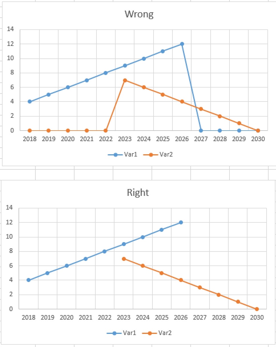
Web Often You May Want To Create A Chart In Excel Using A Range Of Data And Ignore Any Cells That Are Equal To Zero.
Click on the file tab. In the format code box,. Click hidden and empty cells. Select custom in the category box.
Web Use A Number Format To Hide Zero Values In Selected Cells.
If your list of numbers. Web sometimes you might simply want to hide any zero values from your chart, preventing them from appearing at all. Web go to chart tools on the ribbon, then on the design tab, in the data group, click select data. Web choose the number category in the format data labels dialog box.
Web =Na () That Just Needs To Be Incorporated Into The Formula To Say That If The Sum Is Equal To 0, An Na Value Is Returned:
Follow this procedure to hide zero values in selected cells. Web the stacked one, will not ignore the 0 or blank values, but will show a cumulative value according with the other legends. Web on the data tab, click filter in the sort & filter group, to add a filter to all of the columns. The easiest way to do this is.